Ac-225 Advanced PSF Modeling (SIMIND)

This tutorial uses the PSF operators obtained using the SPECTPSF toolbox to reconstruct Ac225 data. The operator was obtained using tutorial 5, available at this link. Use of this operator requires the SPECTPSFToolbox to be installed; instructions for installing can be found on the README here

import os
import torch
import dill
import pytomography
from pytomography.io.SPECT import simind
from pytomography.projectors.SPECT import SPECTSystemMatrix
from pytomography.transforms.SPECT  import SPECTAttenuationTransform, SPECTPSFTransform
from pytomography.algorithms import OSEM
from pytomography.io.SPECT.shared import subsample_projections_and_modify_metadata, subsample_amap
from pytomography.likelihoods import PoissonLogLikelihood
import matplotlib.pyplot as plt

# change to where you saved the data
PATH = '/mnt/mydisk2/pytomo_tutorial_data/SPECT/SIMIND-Jaszak'

Load the SIMIND data. In this case, we’ll use the ground truth scatter from SIMIND.

dT = 2.5 * 60 # seconds per projection
activity_conc = 10 # kBq/L, a very high activity conc for Ac225
CPSpMBq = 17 # an approximate calibration factor

# Specify the isotopes and equilibirum ratios based on Bateman equations
isotopes = ['ac225', 'bi213', 'fr221', 'tl209']
isotopes_ratios = [1,1,1,0.0209]
# look at the .h00 files; there are many E windows simulated. These are 5% scat win for 440peak
i_peak, i_lower, i_upper = 10, 11, 14
files_NM = [[os.path.join(PATH, f'{isotope}', f'tot_w{i}.h00') for isotope in isotopes] for i in [i_lower, i_peak, i_upper]]
object_meta, proj_meta = simind.get_metadata(files_NM[0][0])
activity_concs = [activity_conc * ratio for ratio in isotopes_ratios]
projections = simind.get_projections(files_NM, activity_concs)
projections *= dT

# Based on how they are loaded, this is idx of peak, lower upper
idx_peak, idx_lower, idx_upper = 1, 0, 2
photopeak = projections[idx_peak]
ww_lower, ww_peak, ww_upper = [simind.get_energy_window_width(path) for path in [files_NM[0][0], files_NM[0][1], files_NM[0][2]]]
scatter_estimate_TEW = simind.compute_EW_scatter(
    projections[idx_lower], projections[idx_upper],
    ww_lower,
    ww_upper,
    ww_peak,
    sigma_r=0.5,
    sigma_z=0.5,
    proj_meta=proj_meta
)

We’re reconstructing the 440keV window so we’ll use the 440keV attenuation map

path_amap = os.path.join(PATH, 'attenuation_maps', 'amap440.hct')
amap = simind.get_attenuation_map(path_amap)

The code below reconstructs using OSEM with 50 iterations and 4 subsets

def perform_reconstruction(psf_transform):
    att_transform = SPECTAttenuationTransform(attenuation_map=amap)
    system_matrix = SPECTSystemMatrix(
            obj2obj_transforms = [att_transform,psf_transform],
            proj2proj_transforms = [],
            object_meta = object_meta,
            proj_meta = proj_meta)
    likelihood = PoissonLogLikelihood(system_matrix, photopeak, scatter_estimate_TEW)
    algorithm = OSEM(likelihood)
    return algorithm(n_iters=50, n_subsets=4)

Open the PSF operator created in this tutorial

# Note that you may need to create this operator yourself with the SPECTPSFToolbox to match your GPU architecture
with open(os.path.join(PATH, 'ac225_psf_operator.pkl'), 'rb') as f:
    psf_operator = dill.load(f)
psf_operator.set_device(pytomography.device)
psf_transform = SPECTPSFTransform(psf_operator=psf_operator)
recon_1Dfit = perform_reconstruction(psf_transform)

Reconstruct using the Gaussian modeling which doesn’t account for the septal penetration and septal scatter:

path_bi213_prim = files_NM[1][1]
psf_meta = simind.get_psfmeta_from_header(path_bi213_prim)
psf_transform = SPECTPSFTransform(psf_meta)
reconbad = perform_reconstruction(psf_transform)

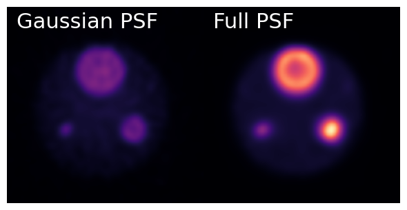
Lets compare the two reconstructions: the first one using the fitted PSF and the second one using the Monte Carlo kernels. Note that the fitted one was over twice as fast for reconstructing!

recons = [reconbad, recon_1Dfit]
titles = ['Gaussian PSF', 'Full PSF']

fig, ax = plt.subplots(1,2,figsize=(6,4), gridspec_kw={'wspace':0.0})
vmax = recons[1].max()
for i in range(2):
    plt.sca(ax[i])
    plt.imshow(recons[i].cpu()[:,:,64].T, cmap='magma', interpolation='gaussian', vmax=vmax)
    plt.text(0.05, 0.87, titles[i], ha='left', va='bottom', fontsize=22, transform=ax[i].transAxes, color='white')
    plt.axis('off')
    plt.xlim(35,95)
    plt.ylim(35,95)
fig.tight_layout()