DICOM Introduction

import os
import numpy as np
from pytomography.io.SPECT import dicom
from pytomography.transforms.SPECT import SPECTAttenuationTransform, SPECTPSFTransform
from pytomography.algorithms import OSEM
from pytomography.projectors.SPECT import SPECTSystemMatrix
from pytomography.likelihoods import PoissonLogLikelihood
from pytomography.utils import print_collimator_parameters
import matplotlib.pyplot as plt
import pydicom
import shutil

# change this to where you downloaded the SPECT tutorial data
PATH = '/mnt/mydisk2/pytomo_tutorial_data/SPECT'
PATH = os.path.join(PATH, 'Lu177-NEMA-SymT2')

Part 1: Opening Data

First we specify the required filepaths to open the SPECT scan (file_NM) and the CT data files (files_CT).

# initialize the `path`` variable below to specify the location of the required data
path_CT = os.path.join(PATH, 'CT')
files_CT = [os.path.join(path_CT, file) for file in os.listdir(path_CT)]
file_NM = os.path.join(PATH, 'projection_data.dcm')

The metadata for object space and projection space can be obtained from the projection data file using dicom.get_metadata

• This contains informaiton such as the voxel size, number of angles, scanner radius, etc.

object_meta, proj_meta = dicom.get_metadata(file_NM, index_peak=0)

We can get the photopeak projection data from the DICOM file provided we know the indices of each of the energy windows. We can obtain that as follows:

dicom.print_energy_window_info(file_NM)

Index 0:   Name: "Window Group A", Energies: [187.19999694824keV, 228.80000305176keV]
Index 1:   Name: "Window Group B", Energies: [166.39999389648keV, 187.19999694824keV]
Index 2:   Name: "Window Group C", Energies: [228.80000305176keV, 249.60000610352keV]
Index 3:   Name: "Window Group D", Energies: [101.69999694824keV, 124.30000305176keV]
Index 4:   Name: "Window Group E", Energies: [85.879997253418keV, 101.69999694824keV]
Index 5:   Name: "Window Group F", Energies: [124.30000305176keV, 146.89999389648keV]

In this case, since we are specifically imaging the 208 keV peak, we specify index_peak=0, so it only returns the projections corresponding to the 187-228 energy window above.

photopeak = dicom.get_projections(file_NM, index_peak=0)
photopeak.shape

torch.Size([96, 128, 128])

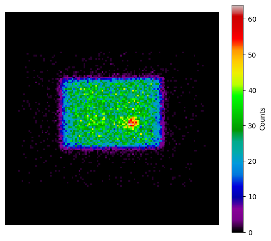
The shape of the photopeak is \((N_{angles}, \text{Width}, \text{Height})\).

plt.figure(figsize=(7,6))
plt.imshow(photopeak[0].cpu().T, cmap='nipy_spectral', origin='lower')
plt.axis('off')
plt.colorbar(label='Counts')

<matplotlib.colorbar.Colorbar at 0x78ed2e5a8a70>

Scatter projections can be estimated using the triple energy window function dicom_get_scatterTEW. One needs to specify the index of the peak, and lower/upper energy windows

scatter = dicom.get_energy_window_scatter_estimate(file_NM, index_peak=0, index_lower=1, index_upper=2)

Part 2: Modeling

Attenuation Transform

The attenuation transform is used to “correct” for the fact that some photons get atteunated in the patient before they reach the detector. PyTomography has functionality to do attenuation correction provided either (i) an argument attenuation_map=... OR (ii) an argument filepath=... is provided to the SPECTAttenuationTransform.

• attenuation_map must be aligned with the SPECT projection data and have units of cm \(^{-1}\) .

• filepath specifies the directory of some CT scan which will be used for attenuation correction. PyTomography has functionality to align this with the SPECT projections and convert to units of cm \(^{-1}\).

In this case, since we’re reconstructing DICOM data, it’s easier to use filepath than to manually align/rescale the CT data

att_transform = SPECTAttenuationTransform(filepath=files_CT)

If we want to view the attenuation map, we need to configure the att_transform so that (i) the CT data can be aligned with SPECT projection data and (ii) the CT data can be converted to attenuation coefficients.

• Note: This is not required if you don’t want to view the attenuation map. Later, when the system matrix is built, it automatically configures all the transforms

att_transform.configure(object_meta, proj_meta)
attenuation_map = att_transform.attenuation_map

Given photopeak energy 208.0 keV and CT energy 130 keV from the CT DICOM header, the HU->mu conversion from the following configuration is used: 208.0 keV SPECT energy, 130 keV CT energy, and scanner model symbiat2

Viewing the attenuation map allows for a consistency check to ensure that it’s properly aligned with the projection data

sample_slice = attenuation_map.cpu()[:,70].T

plt.subplots(1,2,figsize=(7,3))
plt.subplot(121)
plt.title('Projection Data')
plt.imshow(photopeak[0].cpu().T, cmap='nipy_spectral', origin='lower')
plt.axis('off')
plt.colorbar(label='Counts')
plt.subplot(122)
plt.title('From CT Slices')
plt.imshow(sample_slice, cmap='Greys_r', origin='lower', interpolation='Gaussian')
plt.axis('off')
plt.colorbar()

<matplotlib.colorbar.Colorbar at 0x78ed2c33f6e0>

PSF Modeling

PSF modeling requires knowing the parameters of the collimators used for the scan. A list of all supported collimator types can be determined by uncommenting the following line and running it

#print_collimator_parameters()

In our case, we know that this scan was performed on a Siemens Symbia scanner with medium energy collimators and 3/8’’ crystals

• There is an option to use intrinsic resolution of the crystals of the scanner (if you know it); this has a minor impact on the reconstruction

collimator_name = 'SY-ME'
energy_kev = 208 #keV
intrinsic_resolution=0.38 #mm
psf_meta = dicom.get_psfmeta_from_scanner_params(
    collimator_name,
    energy_kev,
    intrinsic_resolution=intrinsic_resolution
)
print(psf_meta)

kernel_dimensions = 2D
min_sigmas = 3
shape = gaussian
sigma_fit_params = [np.float64(0.03161982627275948), np.float64(0.1248503046423388), np.float64(0.16137114205472364)]

Now we can build our PSF transform required to create the system matrix

psf_transform = SPECTPSFTransform(psf_meta)

System Matrix

Now that we have the required transforms, we can begin to build the system matrix. It requires:

1. obj2obj_transforms. These map from object space to object space. In the case of SPECT imaging, both the attenuation transform and PSF transform correspond to these types of transforms.

2. proj2proj_transforms: These map from projection to projection space. Though we have none here, they would be used to model PSF in PET imaging.

3. object_meta and proj_meta. These are used to initialize the transforms. For example, data from object_meta is used to align the attenuation map, and radial position from proj_meta is used to get proper blurring parameters for the PSF transform

system_matrix = SPECTSystemMatrix(
        obj2obj_transforms = [att_transform,psf_transform],
        proj2proj_transforms = [],
        object_meta = object_meta,
        proj_meta = proj_meta)

Given photopeak energy 208.0 keV and CT energy 130 keV from the CT DICOM header, the HU->mu conversion from the following configuration is used: 208.0 keV SPECT energy, 130 keV CT energy, and scanner model symbiat2

The system matrix \(H\) represents the imaging system and maps an object \(f\) to a corresponding image \(g\) under the imaging system

Likelihood

likelihood = PoissonLogLikelihood(system_matrix, photopeak, scatter)

Reconstruct the object

We’ll reconstruct the object using OSEM. For this, we need to specify the measured projection data (photopeak/scatter) and the system_matrix

reconstruction_algorithm = OSEM(likelihood)

We can reconstruct the object by calling the reconstruction algorithm for a given number of iterations/subsets.

reconstructed_object = reconstruction_algorithm(n_iters=4, n_subsets=8)

We can compare this reconstruction to one done by the vendor:

• Note: we divide the vendor reconstruction by 96 because this particualr vendor multiplies by the number of acquisition angles when saving the data. (some vendors alternatively divide by 48, the number of projection angles, so be careful)

ds_recon = pydicom.dcmread(os.path.join(PATH, 'scanner_recon.dcm'))
recon_vendor = ds_recon.pixel_array / proj_meta.num_projections
recon_vendor = np.transpose(recon_vendor, (2,1,0))

We can looks at axial slices from all three reconstructions.

idx_z = 61
slice_pytomography = reconstructed_object.cpu()[:,:,idx_z].T
slice_vendor = recon_vendor[:,:,idx_z].T

plt.subplots(1,2,figsize=(7,3), gridspec_kw={'wspace':0.0})
plt.subplot(121)
plt.imshow(slice_pytomography , cmap='magma', vmax=27, interpolation='gaussian', origin='lower')
plt.text(0.03, 0.97, 'PyTomography', color='white', fontsize=12, fontweight='bold', transform=plt.gca().transAxes, ha='left', va='top')
plt.xlim(30,98)
plt.ylim(98,40)
plt.axis('off')
plt.subplot(122)
plt.imshow(slice_vendor, cmap='magma', vmax=27, interpolation='gaussian', origin='lower')
plt.text(0.03, 0.97, 'Siemens Software', color='white', fontsize=12, fontweight='bold', transform=plt.gca().transAxes, ha='left', va='top')
plt.xlim(30,98)
plt.ylim(98,40)
plt.axis('off')
plt.show()

Saving Data

PyTomography has functionality for saving DICOM data. There are a few things required:

1. The folder where you want to save the data. The folder can’t exist already (has to be a new folder); this prevents overwriting potential data.

2. The reconstructed object itself: in this case, recon_CTslices

3. The filepath of the projection data file_NM. Much of the study/patient information is copied over from this file to the reconstructed file.

4. An optional string that represents the type of reconstruction performed. If left blank, will be an empty string ''

Note: Some vendor reconstructions (i) multiply by the total number of projections and/or (ii) normalize to counts/second when they save their SPECT reconstructions. Make sure to multiply ``reconstructed_object`` by these values before you save if you want to do such comparisons.

# Modify the path below to a location on your computer where you want to save the data
save_path = os.path.join(PATH, 'SPECT', 'Pytomo-Recon')
# Code only works if folder doesnt exist, so delete it if present
if os.path.exists(save_path) and os.path.isdir(save_path):
    shutil.rmtree(save_path)
# Save
dicom.save_dcm(
    save_path = save_path,
    object = reconstructed_object,
    file_NM = file_NM,
    recon_name = 'OSEM_4it_8ss')

The data can now be exported to any DICOM viewer of your choice!